
Use of the characteristic (density) curve with an exposure chart
How do I use the characteristic (density) curve with an exposure chart?
In the following examples the tube voltage and focus-to-film distance (FFD) are assumed to be constant, and automatic development is for 8 minutes in G135 developer at 28°C.
Example 1:
Effect of the thickness of the object on the density of the radiographic image
It is required to radiograph, on D7 film, a steel object comprising two sections of different thickness of 12 mm and 15 mm. The exposure chart figure 7-9 shows that at 160 kV and an FFD. of 70 cm, using 10mA.min, a density of 2 behind the section measuring 15 mm in thickness will be obtained.
Question: What image density will be obtained behind the section measuring 12 mm under these given conditions?
Method and answer
The exposure chart (fig.7-9) shows that under the conditions mentioned above density D = 2 is obtained on D7-film through the 15 mm thick section, using an exposure of 10 mA.min, point A on the chart.
Under the same conditions the 12 mm section would require an exposure of 5 mA.min (point B in the chart), which means an exposure ratio of 10/5. The exposure through the 12 mm section is two times greater than through the 15 mm section. The logarithm of this ratio equals: 0.3 (log 2 = 0.3).
The characteristic curve (fig. 8-9) of the D7-film shows that density 2 corresponds to log relative exposure 2.2 (point C in fig. 8-9). At 12 mm the log. rel. exposure is 2.2 + 0.3 = 2.5. The corresponding density is then 3.5 (point D in fig. 8-9).
Example 2:
Effect of exposure on contrast
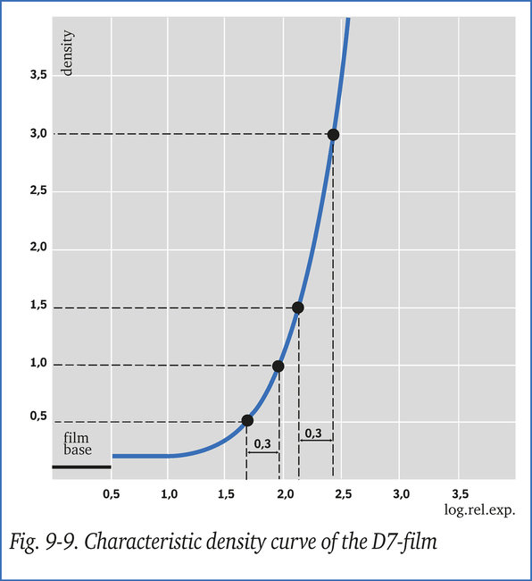
Assume that when an exposure of 15 mA.min is used for a radiograph on D7-film, both average density and contrast prove to be too low after processing. The highest and lowest density in the most relevant section of the image are only 1.5 and 0.5. The intention was to make a radiograph with a maximum density of 3.0.
Questions: What exposure time would be required for the same radiation intensity and what contrast increase would be achieved?
Method and answer
The characteristic curve (fig. 9-9) shows that at the measured densities of 1.5 and 0.5 respectively, the corresponding logarithm of relative exposures are 2.15 and 1.65.
Since density 3.0 should not be exceeded, the area which is most important for interpretation, which showed density 1.5 on the first exposure, must now display 3.0 Characteristic curve, figure 9-9, shows that density 3.0 corresponds with log.rel.exp. 2.45 and the difference between the two values amounts to 2.45 - 2.15 = 0.3.
This means that the exposure time must be doubled (100.3 = 2), resulting in a radiation dose of 30 mA.min. This answers the first question.
If the exposure time is doubled, the log.rel.exposure of the lowest density value originally measured will increase by 0.3, i.e. 1.65 + 0.3 = 1.95. The corresponding density will be 1.0 (fig. 9-9).
The average gradient between the upper and lower densities on the original radiograph was (1.5 - 0.5) / (2.15 - 1.65) = 2.0. The average gradient on the new radiograph is (3.0 - 1.0) / (2.45 - 1.95) = 4.0, so the average contrast has doubled.